This vignette demonstrates how to perform uniform manifold approximation and projection (UMAP), add the resulting UMAP coordinates to an NG-CHM, and explore the interactive features between dimensionality reduction plots and the NG-CHM via the 2D Scatter Plot Plugin. A similar analysis can be performed for use with the 3D Scatter Plot Plugin.
Uniform Manifold Approximation and Projection (UMAP)
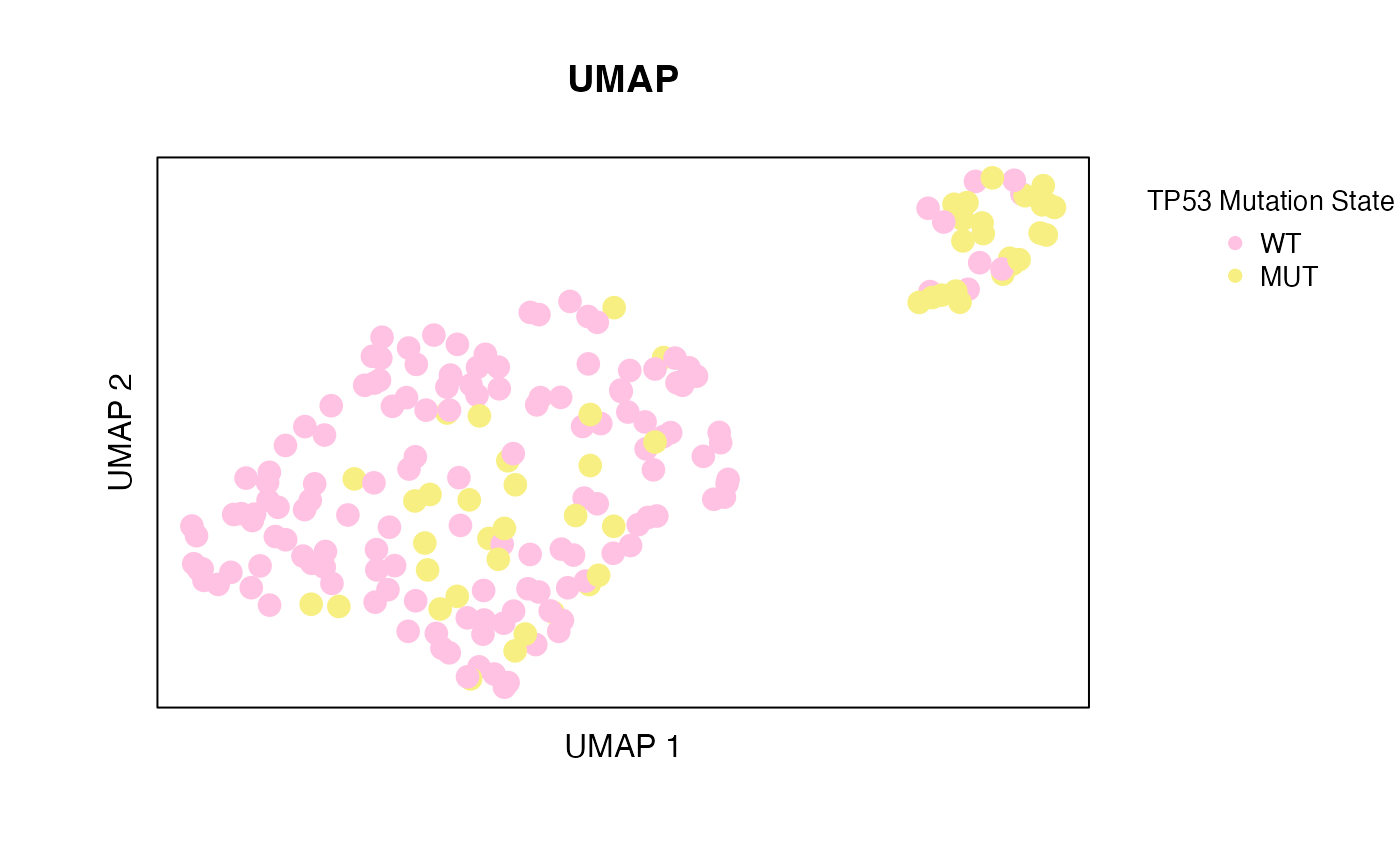
The code block below reads in the NGCHMDemoData, performs principal component analysis (PCA), and calculates UMAP coordinates from the principal components. This vignette uses the umap R package which must be installed in order to run the code below. (See Getting Started for details on creating NG-CHMs). A static plot of the UMAP coordinates, colored by TP53 mutation state is displayed in Figure 1.
PCA was performed first because it yielded better group separation compared to performing UMAP on the raw data.
# Read in NGCHMDemoData (as in the Getting Started vignette)
library(NGCHMDemoData)
matrix_data_file <- system.file("extdata", "TCGA.BRCA.Expression.csv", package = "NGCHMDemoData")
matrix_data <- as.matrix(read.csv(matrix_data_file, header = TRUE, row.names = 1, check.names = FALSE, stringsAsFactors = FALSE))
covariate_data_file <- system.file("extdata", "TCGA.BRCA.TP53Mutation.csv", package = "NGCHMDemoData")
covariate_data <- read.csv(covariate_data_file, row.names = 1, check.names = FALSE, stringsAsFactors = FALSE) # read.csv returns a data.frame
covariate_vector <- covariate_data[["MutationState"]] # create vector
names(covariate_vector) <- rownames(covariate_data) # set the names
# Calculate principal components
pca_data <- prcomp(as.data.frame(t(matrix_data)), scale = TRUE, center = TRUE, rank = 10)
# Calculate UMAP from principal components
library(umap)
config <- umap::umap.defaults
config$n_neighbors <- 15 # change default for better group separation
config$random_state <- 123 # set random state for reproducibility
umap_data <- umap::umap(pca_data$x, config = config)
Click to expand R code used to create static plot in Figure 1
# Create static plot of UMAP coordinates colored by TP53 mutation state
par(mar = c(4, 4, 4, 8) + 0.1, bg = "white", mgp = c(0.5, 1, 0))
xlim <- range(umap_data$layout[,1])
ylim <- range(umap_data$layout[,2])
plot(xlim, ylim,
     xlab = "UMAP 1",
     ylab = "UMAP 2",
     main = "UMAP",
     type = "n", xaxt = "n", yaxt = "n")
labels_for_point_color <- as.factor(covariate_vector) # "MUT' and "WT"
colors <- c("#f7ef81", "#ffc2e2") # plot only needs two colors: one for "MUT" and one for "WT"
points(umap_data$layout[,1], umap_data$layout[,2],
       col = colors[as.integer(labels_for_point_color)],
       pch = 19, cex = 1.5)
legend(x = xlim[2] + (xlim[2] - xlim[1]) * 0.1, # calculate x position for legend
       y = ylim[2], # calculate y position for legend
       legend = as.character(unique(labels_for_point_color)),
       col = colors[as.integer(unique(labels_for_point_color))],
       title = "TP53 Mutation State",
       inset = 0.03, xpd = TRUE, bty = "n", pch = 19, cex = 0.85)
Figure 1. UMAP plot of TCGA BRCA data colored by TP53 mutation state
Add UMAP to NG-CHM
This section describes how to add the UMAP coordinates calculated above to the NG-CHM such that they can be explored interactively via the 2D Scatter Plot plugin.
Create an NG-CHM
This code block creates an NG-CHM from the data read in above and creates a covariate bar for the TP53 mutation state. The colors of the TP53 mutation state are chosen to match the colors in the UMAP plot above.
library(NGCHM)
hm <- chmNew("TCGA BRCA Expression", matrix_data)
colors <- c("#f7ef81", "#ffc2e2") # same colors as in Figure 1
mutationColorMap <- chmNewColorMap(c("MUT", "WT"), colors)
covariateBar <- chmNewCovariate("TP53 Mutation State", covariate_vector, mutationColorMap)
hm <- chmAddCovariateBar(hm, "column", covariateBar)
Add UMAP Coordinates
The UMAP coordinates are added to the NG-CHM via the convenience
function chmAddUMAP(). Similar functions exist for adding
PCA, TSNE, etc. See the “Add Scatter Plot Coordinates” section on the Function
Reference page for more details. UMAP coordinates can also be added
in a fashion similar to the TP53 mutation state.
hm <- chmAddUMAP(hm, "column", umap_data)
chmExportToHTML(hm, "umap.html", overwrite = TRUE) # create HTML file of NG-CHM
Interactive UMAP / NG-CHM
This section describes how to use the NG-CHM Viewer to explore the UMAP data interactively. NG-CHMs include several plugins, among them a 2D Scatter Plot to allow for interactive exploration of 2-dimensional data. Below are the steps to open this plugin and use it to explore the UMAP coordinates.
It may be helpful to click the “Open NG-CHM in a New Tab” button below and follow these steps in the larger space of a new tab.
- In the “Heat Map Summary” panel, click the button to open the panel menu.
- In the newly opened panel menu, under , select “”.
- In the newly created empty panel, click the button, and under , select “”. This will automatically open the menu for that panel.
- In the newly opened menu, keep the default choices.
- At the bottom of the open menu, click and then .
The UMAP scatter plot should be visible in the lower right panel of the NG-CHM display.
Here are some suggestions for exploring the interactive features between the UMAP plot and the NG-CHM:
- In the 2D Scatter Plot Panel:
- Use the slider to increase the size of the points
- Click the lasso button to enter Lasso/Select mode
- Draw a lasso around a cluster of points
- This will select the corresponding columns in the Heat Map Detail panel
- In the Heat Map Detail Panel:
- Click on a column dendrogram
- This will highlight the corresponding points in the UMAP plot
- Scroll over the Detail Map to zoom enough to see column labels at
the bottom and click on a column label
- This will highlight the corresponding point in the UMAP plot
- Click on a column dendrogram
- Click the button to clear selections.
Further Reading
Additional examples and information are available in Introduction to Creating Single-Cell Next-Generation Clustered Heat Maps in R.